Model Framework - Custom Degradation Profile
Degradation Profiles
The Degradation Profile is the foundation of Strategic Asset Life Cycle modelling.
Assets typically start off as brand new (service state 0), and at some future point in time, the asset will have transitioned to end of life (service state 6).
To model this process we therefore define life cycle degradation profiles, simulating an asset's degradation (the way it moves from one service state to another throughout its life cycle). This is one of the most important steps in Brightly Predictor. The life cycle degradation profiles configured in Predictor describe the relationship between useful life, remaining life, service potential and native scaling (which are all assigned to a Service State) of an asset.
The following explains the relationship between service state, remaining life, service potential and native scale, which are all integral to configuring life cycle degradation profiles.
Service State is a numerical integer value between 0 to 6, which reflects the measure of the condition, performance, physical integrity, health or similar measure of an asset or asset component consistent with the International Infrastructure Management Manual (IIMM) and ISO 55000 guidelines. The life cycle degradation profile describes the relationship between useful life and remaining useful life (assigned to each Service State) of an asset. In essence, the Service State reflects where an asset or asset component is within its defined useful life at any given point in time.
Service Potential is defined in the IIMM as “the total future service capacity of an asset. It is normally determined by reference to the operating capacity and economic life of an asset”. In simple terms, the Service Potential expresses the available service level that the asset or asset component will provide.
Whilst Service State reflects where an asset or asset component is within its defined useful life at any given point in time, the corresponding Service Potential reflects the remaining available service level. In the absence of historical and/or existing Service Potential performance data, generally to begin with and when configuring the degradation profile, ‘Service Potential %’ is aligned to reflect the ‘Remaining Life %’ and hence the values are the same.
Native Scale offers organizations the ability to measure the Service State values using a scale that is ‘native’ to the organization. For example, ASTM D 6433-03 (commonly used in North America) defines the pavement condition index (PCI) as a numerical rating between 0 to 100 where 0 is the worst possible condition and 100 as the best possible condition.
Configuring Degradation Profiles
Predictor contains 13 preconfigured default degradation profiles which can be used to model the Life Cycle degradation profile of an asset, and also allows for users to add and configure their own degradation profiles.
This can be done by navigating to the Degradation Profile tab in the Model Framework section of a Model.
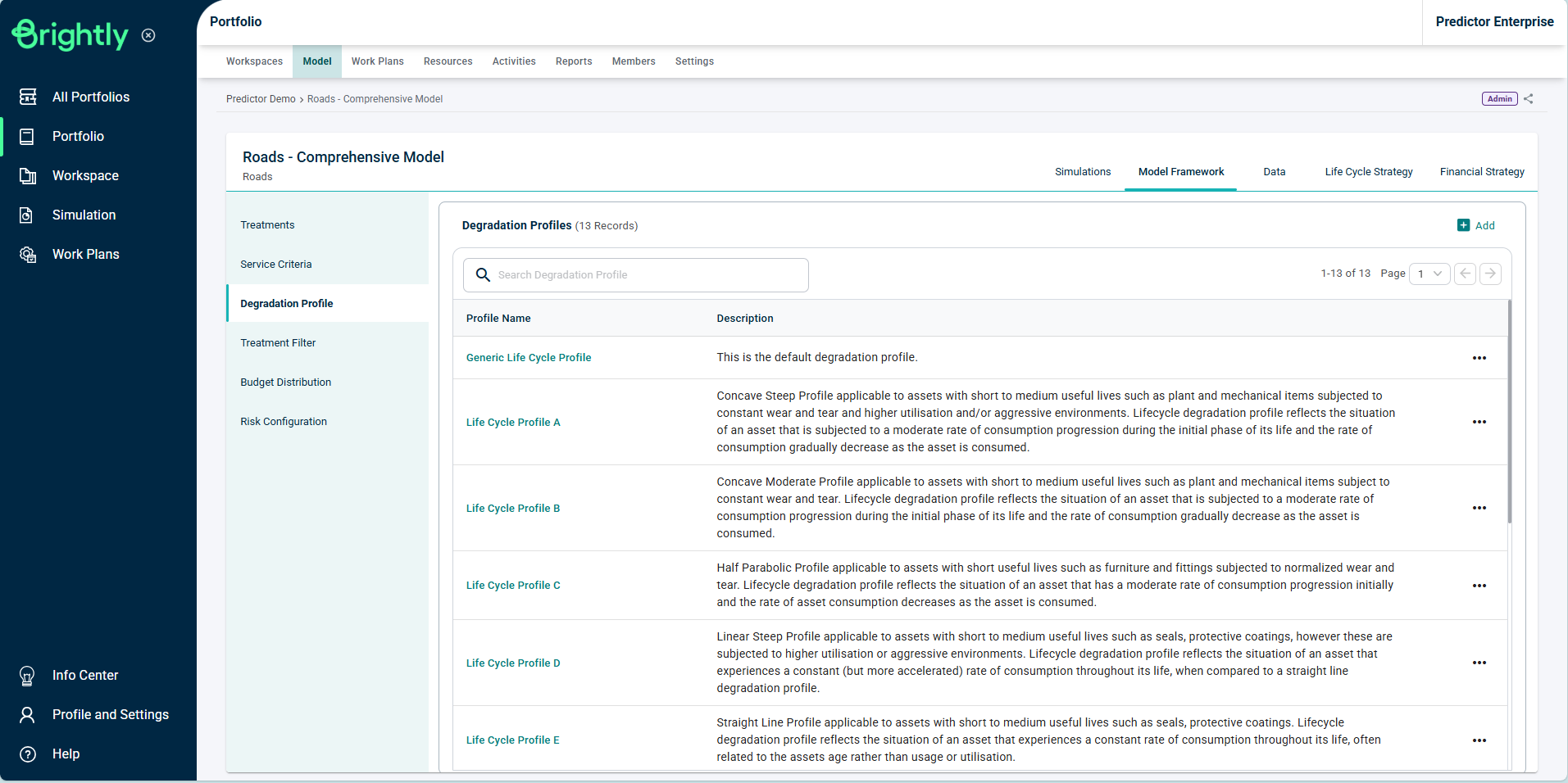
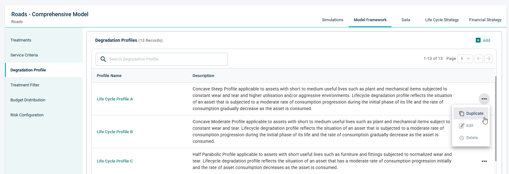
Degradation Profiles can be duplicated by selecting the three-dot menu to the right of a profile in the list.
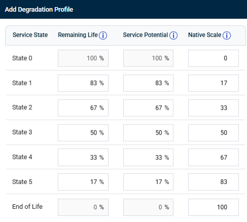
Degradation Profiles can be modified by selecting the name of the profile, and new degradation profiles are added using the ‘Add’ button.
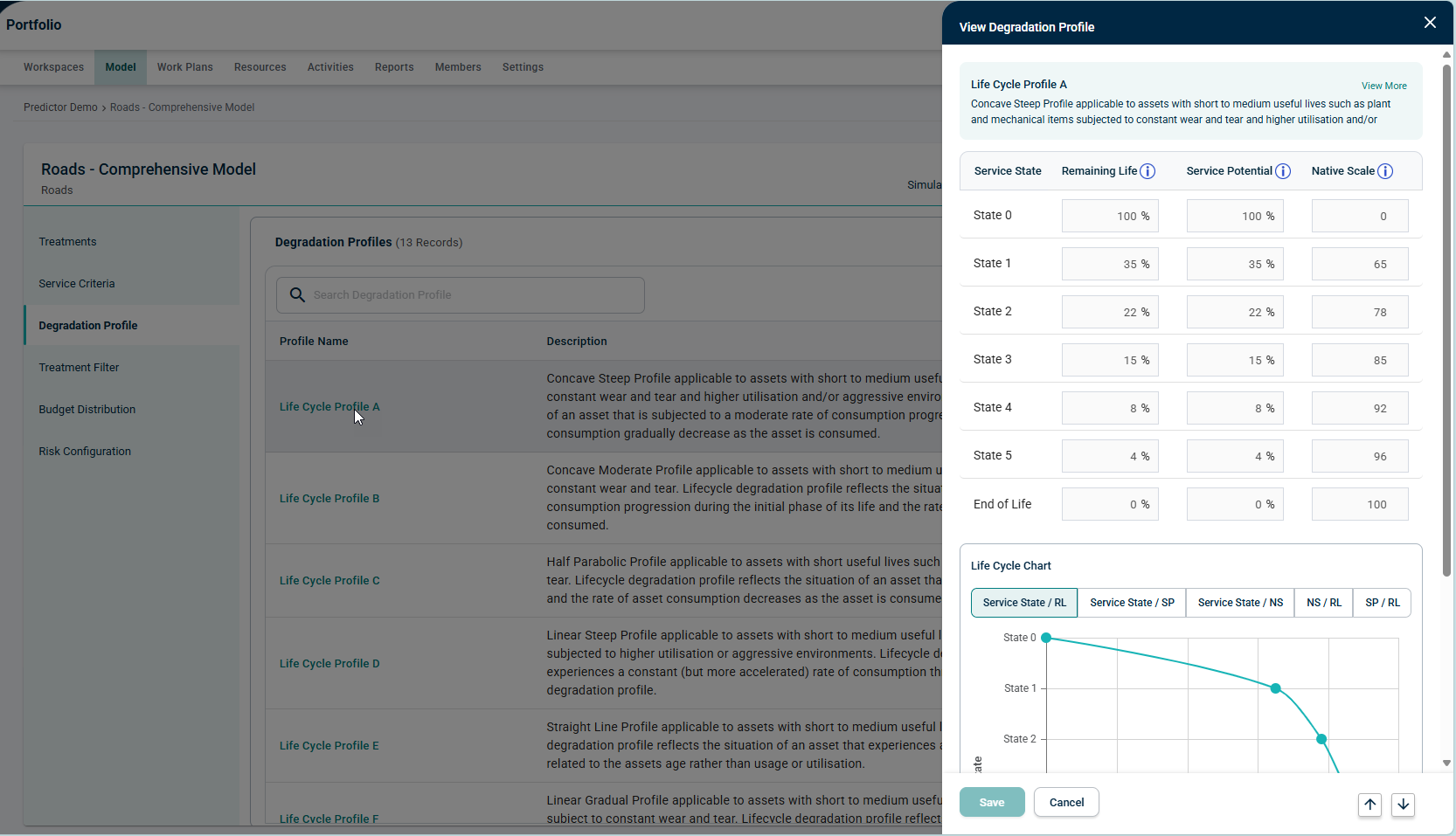
The Remaining Life percentage and Service Potential percentage values are configurable for each condition state by selecting the appropriate cell and inputting a value, which must be less than the previous state. Remaining Life is expressed as a percentage value between 0% and 100% where 0% indicates no life available and 100% represents full life available.
Service Potential is also expressed as a percentage value between 0% and 100%, where 0% indicates no Service Potential and 100% represents full Service Potential available.
Native Scale must always have a maximum value and a minimum value and must be between any two whole number values. However, the scale can be defined in either descending or ascending order.
Some examples of user-defined Native Scale ranges are as follows:
-
0-100
-
100-0
-
1-10
-
10-1
-
0-500
The default native scale values in the pre-configured fixed degradation profiles reflect the 0-100 range and are calculated for each service state using the following equation; 100-Service Potential%.
The Degradation Profiles for a Model will be available when configuring the Life Cycle.