Objective: Gain an understanding of how to use Predictor's Results Feed simulation export functionality in conjunction with ArcGIS.
Introduction
For each Simulation, Predictor Web App provides an in-built functionality that allows for the generation of a Simulation Export.
This article outlines the steps for using a Predictor Simulation Export to upload the simulation data to ArcGIS Enterprise. The Simulation results are uploaded as a table that can then be joined to your spatial layers for visualisation. If you intend to append the simulation results to a spatial layer ensure you have a spatial layer prepared that contains a unique ID reference to the simulation.
There are two options for accessing the export:
- The end-user is able to download the Simulation Export as a CSV file as per the article Simulation Export
- The end-user is able to create a sharable Results Feed link for the Simulation Export. The link can be used as a data source for ArcGIS Enterprise (ArcGIS Online or Portal for ArcGIS). This link does not require a login to Predictor and can therefore be sent to another user to access.
- The Results Feed article outlines how to access the Results Feed Simulation Export Link.
There are two applications available for making the Predictor Simulation result available in ArcGIS Enterprise:
- The ArcGIS Enterprise browser interface
- ArcGIS Pro
Prior to utilising the Predictor Simulation Export in ArcGIS Enterprise the Predictor Simulation Export may optionally be edited to suit final requirements.
Prepare Simulation Export for upload
Time Series
If you want to present the Predictor Simulation results as a time series layer then users will need to add 2 date columns to the simulation export. Otherwise, skip this step.
First, use the Results Feed Link URL to download the csv file and open in Excel
Next add a ‘Start Date’ and ‘End Date’ column to the Predictor Simulation result data.
Populate the dates as the year start and end dates based on the ‘Year’ column. Note that the year column is relative rather than absolute.
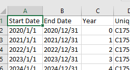
Formula for Start Date (cell A2): =TEXT(2020 + C2,"0") & "/1/1"
Formula for End Date (cell B2): =TEXT(2020 + C2,"0") & "/12/31"
The data format of these columns can remain as ‘General’ since the csv file needs to retain the formatting as YYYY/MM/DD for uploading to ArcGIS Enterprise
Unwanted Columns
The Predictor Simulation results export may include data columns you do not require in ArcGIS Enterprise. It is easiest to remove these columns at this stage of the process.
Upload Simulation using ArcGIS Enterprise
ArcGIS Enterprise provides the complete set of tools required for uploading the Predictor Simulation results, joining to an existing spatial layer, and presenting in a map.
Upload Steps
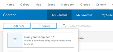
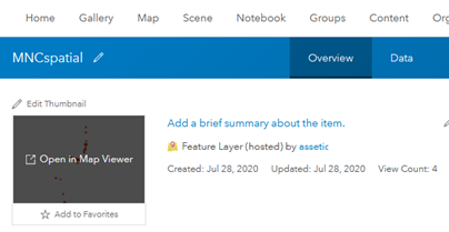
Log in to ArcGIS Enterprise and navigate to Content -> My Content
Initiate Simulation upload
Choose the ‘Add Item’ button, and then choose the ‘From your computer’ option.
From the ‘Add an item from your computer’ dialog choose the ‘browse’ button.
If you have already downloaded the Predictor Simulation results file navigate to the file via the ‘File Upload’ dialog window.
If you haven’t already downloaded the Predictor Simulation results file then in the ‘File Upload’ dialog window paste the Predictor Simulation Results Feed URL into the ‘Filename’ box and then click the ‘Open’ button’.
The file upload will begin. Depending on the Simulation file size this may take several minutes and users are required to wait for all progress dialogs to complete.
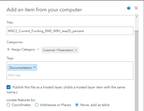
Set Table Name
Define the table name (title) for the Simulation, define any relevant ‘Categories’ and Tags. Note that a tag is mandatory and helps filter content in ArcGIS Enterprise.
NB: The title of a service may only contain alphanumeric characters or underscores and be 120 characters or less.
In this example the title is ‘MNC2_Current_Funding_BMS_WBV_less25_percent.’
Choose the option to ‘Publish this file as a hosted layer.’
For the ‘Locate features by’ choose the option ‘None, add as table’ option.
Finally click on the ‘Add Item’ button at the bottom of the dialog window (not visible in the screenshot below).
Once the ‘Add Item’ button is selected, ArcGIS Enterprise will start to create the feature service with the table. This may also take several minutes. The browser page will automatically navigate to the new feature service when it starts to create the new service. Once complete the service can be utilised.
Join Simulation Result Table to Spatial Layer
To visualise the Predictor Simulation results spatially the uploaded table is joined to an existing spatial layer in ArcGIS Enterprise. The result of the join can be either a View or a new feature layer.
Note that a View does not consume credits in the creation process or as storage. For a large table, a Feature Layer may provide better performance.
In ArcGIS Enterprise, navigate to the feature layer containing the spatial data and open the layer in the ‘Map Viewer’.
In the ‘Map Viewer’ choose the menu option ‘Analysis’, expand the menu ‘Summarize Data.’
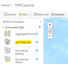
Choose ‘Join Features’ to define the join parameters.
- Target Layer: This is the spatial layer
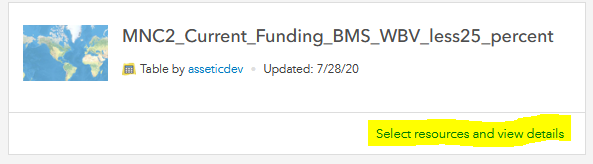
- Layer to join to target layer is the Predictor Simulation result table. Choose the option ‘Choose Analysis Layer’ from the dropdown.
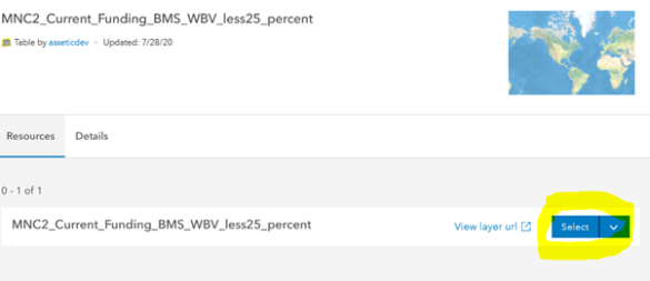
Then navigate to and choose ‘Select resources and view details’ for the uploaded Predictor Simulation Result table.
And then choose ‘Select.’
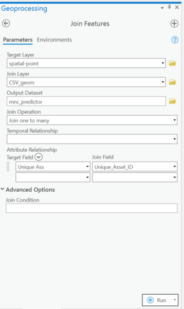
- The ‘type of join’ defaults to field match. The spatial layer needs to have a Unique Id field that also exists in the Predictor Simulation Result table.
- Target Field: The unique identifier in the spatial layer
- Join Field: The field in the Predictor Simulation Result table corresponding to the unique Id in the spatial table. Usually, this is the ‘Unique_Asset_Id’ in the Predictor Simulation Result table
- Join Operation: This is ‘join one to many’ because for each asset the Predictor Simulation result will have multiple records representing the result for each year of the simulation
- Tick “Keep all target features” if you want all features in the spatial layer to be in the view regardless of whether there is a corresponding record in the Simulation Results table
- Result Layer Name is the name of resultant View or Feature Service.
- The folder to save the result in can be specified
- Tick ‘Create results as hosted feature layer view’ to create a view, or else a Feature Service is created. If creating a Feature Service the number of credits required to create the Feature Service can be viewed via the ‘Show Credits’ link.
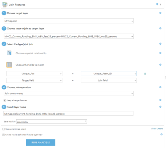
Click on the ‘Run Analysis’ button to create the View Feature Service or Feature Layer Service. Note that this may take several minutes to complete depending on the number of features and the number of records in the Predictor Simulation results.
Configure Resultant Layer
The generated feature layer/view can be configured as a time series layer and have symbology representing asset OSI.
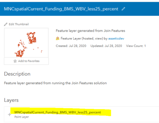
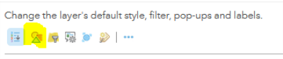
The newly created layer will be added to the Map Viewer legend. To access the Feature Service containing the layer, click on the layer options and choose ‘Show Item Details’.
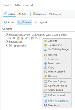
Next, navigate to the layer by clicking on it in the layer list (highlighted in the screenshot below).
There are several configurations that may be applied once you are viewing the layer.
Time Series
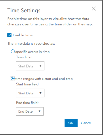
Enable time series for the created layer (MNCspatialCurrent_Funding_BMS_WBV_less25_percent) by editing the time settings.
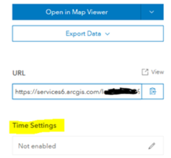
Tick the ‘enable time’ checkbox and then select the option 'time ranges with a start and end time'. Set the start date and date fields to match the date fields added to the Predictor Simulation Export file prior to upload as a table.
Visualization
The layer symbology and other features of layer visualisation can be set via the ArcGIS Enterprise user interface.
Symbology
The symbology of the layer can be set by navigating to the ‘Visualization’ setting for the layer.

Typically, the field |SI|OSI| is used because it represents asset condition and has an integer range of 0 to 6.
Choose the ‘Change Style’ option:
- Select the |SI|OSI| field
- Choose the “Types (Unique symbols)” Drawing Style option
- Set the colour for each of the OSI values and apply, remembering to ‘Save Layer’ once the styles are applied.
Styles
|
OSI |
Hex Identifier |
|
0 |
#61a336 |
|
1 |
#7acc44 |
|
2 |
#addb59 |
|
3 |
#d5d95c |
|
4 |
#f7ae6b |
|
5 |
#e27b69 |
|
6 |
#c4534b |
Point Clustering
If using point data, point clustering can be used when viewing large numbers of records at a large scale. As you zoom in the records gradually de-aggregate. This is a useful method to view problem areas at a large scale and then zoom in to expand the detail.
Applying visualisation via service definition
Instead of using the ArcGIS Enterprise user interface to apply visualisation settings, the settings can be defined in the layer service definition. The service definition needs to be opened in 'edit' mode to allow the visualisation settings to be applied.
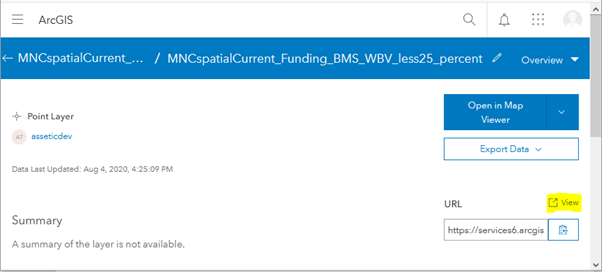
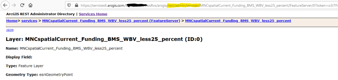
To view the service definition open the layer in ArcGIS Enterprise (not the feature service), and click on the ‘View’ link above the service URL.
The service definition page is initially opened in read-only mode:
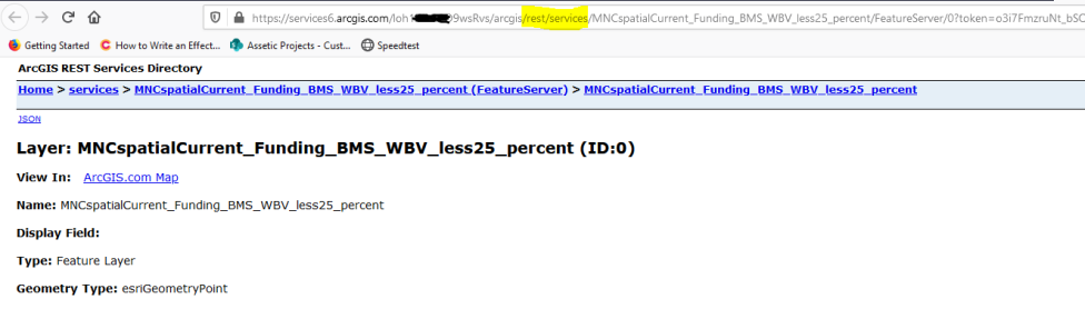
To open the service definition in 'edit' mode, edit the URL of the page to include "admin" between "/rest/services/" i.e. "/rest/admin/services/". This is changed is underlined in the screenshots above and below:
Once in 'edit' mode the service definition option 'Update Definition' should be visible at the bottom of the service definition page:
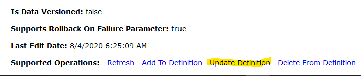
Click on the "Update Definition" link to open the following page:
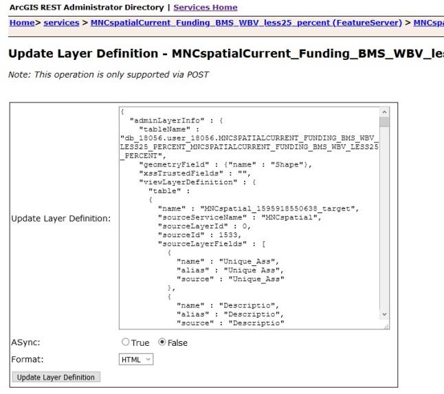
It is on this page that the following updates can be applied via the JSON definitions described below.
Set the time series interval
The time series interval can be set as yearly to match the Predictor Simulation output which is also yearly. ArcGIS Enterprise doesn’t always get the intervals in the time slider right, so setting it as yearly overcomes this issue.
This ESRI blog describes setting the time series interval in detail: https://www.esri.com/arcgis-blog/products/arcgis-online/sharing-collaboration/configuring-time-in-arcgis-online/
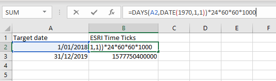
It is necessary to convert the full date range (timeExtent) to ESRI time ticks by multiplying the number of days since 1st January 1970 by 24*60*60*1000. An example conversion is shown in the Excel screenshot below:
In the Update Layer Definition box first delete the current JSON definition and then paste in your JSON definition for "timeExtent" from the sample below
Using the calculated "ESRI Time Tics" from above, edit the JSON definition for "timeExtent" in "timeInfo" and make sure "startTimeField" and "endTimeField" field names match your data.
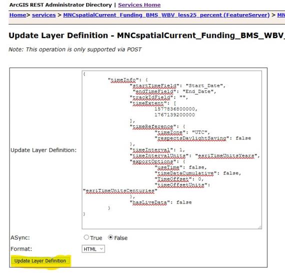
Apply the changes via the "Update Service Definition" button highlighted in the screenshot above:
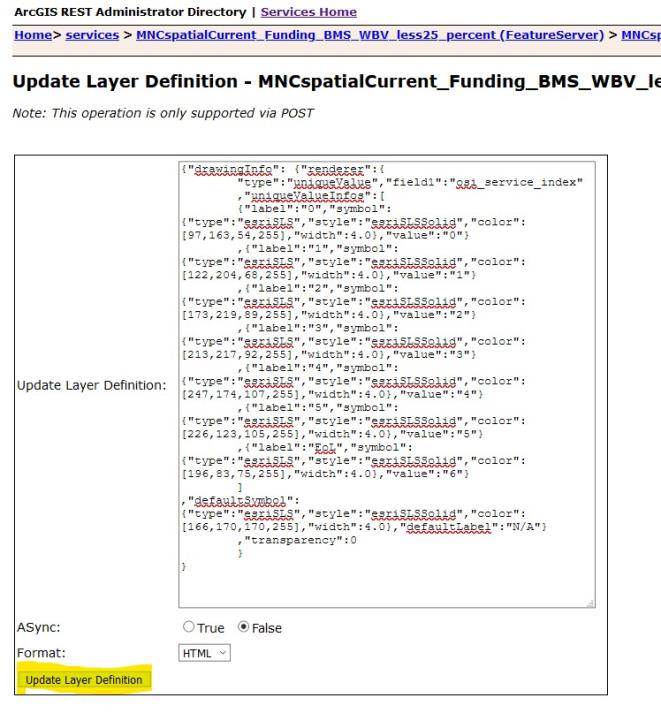
Set the symbology via API
The following JSON definitions can be used to define the symbology of the layer. Using this method is fast and ensures all layers have the same symbology, which is useful when presenting comparison maps.
As with the example above for setting the "timeInfo", open the "Update Definition" page for the layer and clear the current JSON definition in the box adjacent to the label "Update Layer Definition".
The definition differs for each feature type - e.g. Point, Line, or Polygon.
Copy the one of the JSON options from below and paste in the box adjacent to the "Update Service Definition" label. Use the JSON relevant to your layer feature type.
For Polyline Layers:
"type":"uniqueValue","field1":"osi_service_index"
,"uniqueValueInfos":[
{"label":"0","symbol":{"type":"esriSLS","style":"esriSLSSolid","color":[97,163,54,255],"width":4.0},"value":"0"}
,{"label":"1","symbol":{"type":"esriSLS","style":"esriSLSSolid","color":[122,204,68,255],"width":4.0},"value":"1"}
,{"label":"2","symbol":{"type":"esriSLS","style":"esriSLSSolid","color":[173,219,89,255],"width":4.0},"value":"2"}
,{"label":"3","symbol":{"type":"esriSLS","style":"esriSLSSolid","color":[213,217,92,255],"width":4.0},"value":"3"}
,{"label":"4","symbol":{"type":"esriSLS","style":"esriSLSSolid","color":[247,174,107,255],"width":4.0},"value":"4"}
,{"label":"5","symbol":{"type":"esriSLS","style":"esriSLSSolid","color":[226,123,105,255],"width":4.0},"value":"5"}
,{"label":"EoL","symbol":{"type":"esriSLS","style":"esriSLSSolid","color":[196,83,75,255],"width":4.0},"value":"6"}
]
,"defaultSymbol":{"type":"esriSLS","style":"esriSLSSolid","color":[166,170,170,255],"width":4.0},"defaultLabel":"N/A"}
,"transparency":0
}
}
For Point Layers:
{"type":"uniqueValue","field1":"osi_service_index","uniqueValueInfos":[
{"label":"0","symbol":{"type":"esriSMS","style":"esriSMSCircle","color":[97,163,54,255],"angle":0,"size":6},"value":"0"}
,{"label":"1","symbol":{"type":"esriSMS","style":"esriSMSCircle","color":[122,204,68,255],"angle":0,"size":6},"value":"1"}
,{"label":"2","symbol":{"type":"esriSMS","style":"esriSMSCircle","color":[173,219,89,255],"angle":0,"size":6},"value":"2"}
,{"label":"3","symbol":{"type":"esriSMS","style":"esriSMSCircle","color":[213,217,92,255],"angle":0,"size":6},"value":"3"}
,{"label":"4","symbol":{"type":"esriSMS","style":"esriSMSCircle","color":[247,174,107,255],"angle":0,"size":6},"value":"4"}
,{"label":"5","symbol":{"type":"esriSMS","style":"esriSMSCircle","color":[226,123,105,255],"angle":0,"size":6},"value":"5"}
,{"label":"EoL","symbol":{"type":"esriSMS","style":"esriSMSCircle","color":[196,83,75,255],"angle":0,"size":6},"value":"6"}]
,"defaultSymbol":{"type":"esriSMS","style":"esriSMSCircle","color":[166,170,170,255],"angle":0,"size":6}
,"defaultLabel":"N/A"}
,"transparency":0}
}
For Polygon Layers:
"type":"uniqueValue","field1":"osi_service_index"
,"uniqueValueInfos":[
{"label":"0","symbol":{"type":"esriSLS","style":"esriSLSSolid","color":[97,163,54,255],"width":4.0},"value":"0"}
,{"label":"1","symbol":{"type":"esriSLS","style":"esriSLSSolid","color":[122,204,68,255],"width":4.0},"value":"1"}
,{"label":"2","symbol":{"type":"esriSLS","style":"esriSLSSolid","color":[173,219,89,255],"width":4.0},"value":"2"}
,{"label":"3","symbol":{"type":"esriSLS","style":"esriSLSSolid","color":[213,217,92,255],"width":4.0},"value":"3"}
,{"label":"4","symbol":{"type":"esriSLS","style":"esriSLSSolid","color":[247,174,107,255],"width":4.0},"value":"4"}
,{"label":"5","symbol":{"type":"esriSLS","style":"esriSLSSolid","color":[226,123,105,255],"width":4.0},"value":"5"}
,{"label":"EoL","symbol":{"type":"esriSLS","style":"esriSLSSolid","color":[196,83,75,255],"width":4.0},"value":"6"}
]
,"defaultSymbol":{"type":"esriSLS","style":"esriSLSSolid","color":[166,170,170,255],"width":4.0},"defaultLabel":"N/A"}
,"transparency":0
}
}
Paste the JSON definition and click on the "Update Layer Definition" button highlighted in the screenshot below:
Uploading via ArcGIS Pro
If preferred the Predictor Simulation Export file may also be uploaded to ArcGIS Enterprise via ArcGIS Pro.
Import into ArcGIS Pro
The first step is to download the Predictor Simulation Export file as per the section titled ‘Prepare Simulation Export for upload.’
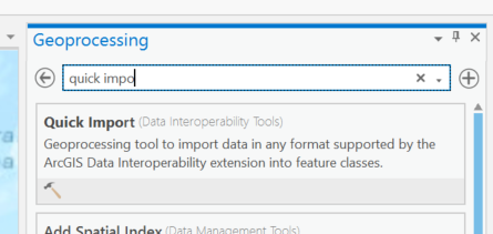
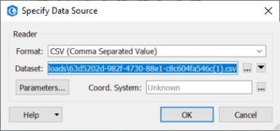
Once completed, the Geoprocessing Tool ‘Quick Import’ can be used to import the Predictor Simulation Export file.
When selecting the source for the ‘Input Dataset’ use the ‘Parameters…’ button to fine-tune the import by excluding unwanted fields (if not already excluded) and ensure data types are correct.
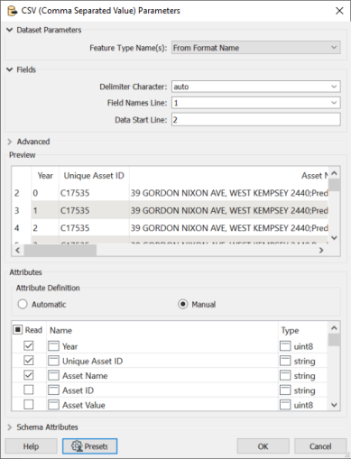
The ‘Presets’ button can be used to save the settings for re-use.
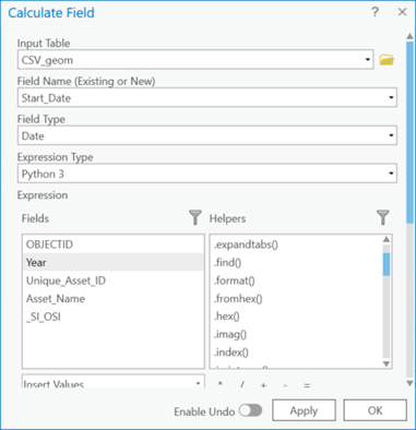
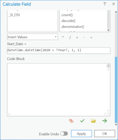
Add Start and End date
To create a time-enabled layer, add a ‘Start Date’ and ‘End Date’ field to the table using the ArcGIS field calculator. Set the field as type ‘Date’ and use Python 3 to calculate the date using the below formulas for start and end dates respectively:
- datetime(2020+!Year!, 1, 1)
- datetime(2020 + !Year!, 12, 31)
Join Predictor Simulation to Spatial Layer
Add the generated table from the Quick Import to a map window containing the spatial layer to merge with the Predictor Simulation result. This is conceptually the same as the section titled ‘Join Simulation Result Table to Spatial Layer.’
Prepare joined layer for upload
The generated layer can be edited prior to upload to ArcGIS Enterprise.
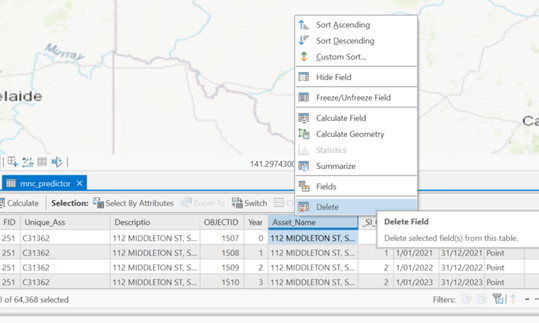
Remove Unwanted Fields
Remove duplicate or unwanted fields by opening the attribute table, right-clicking on unwanted fields and selecting delete. The key field used for linking the Predictor Simulation Results to the spatial layer is an example of a duplicate field. The fewer fields uploaded, the less ArcGIS storage credits required, and potentially the faster the display.
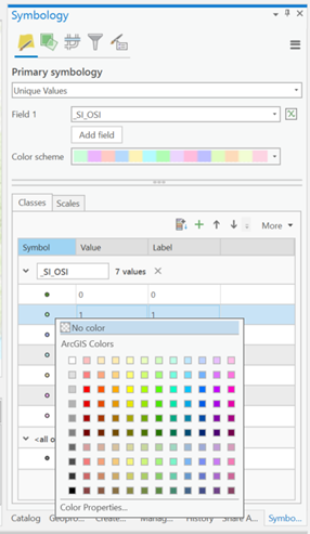
Set Symbology
Choose the type ‘Unique Values’ and then set ‘Field 1’ as the OSI field
There will be 6 unique values plus a default value. For each symbol right-click and choose the ‘Colour Properties’ option. In the ‘colour Editor’ dialog window that pops up enter the ‘HEX’ code listed in the Styles table shown previously. The ‘Save Colour to Style’ option can be used to save the colour for re-use.
The label for ‘6’ is often changed to ‘EoL’ to indicate ‘End of Life’.
An alternative is to set the symbology once uploaded to ArcGIS Enterprise as described in the sections ‘Symbology’ and ‘Set the symbology via API’
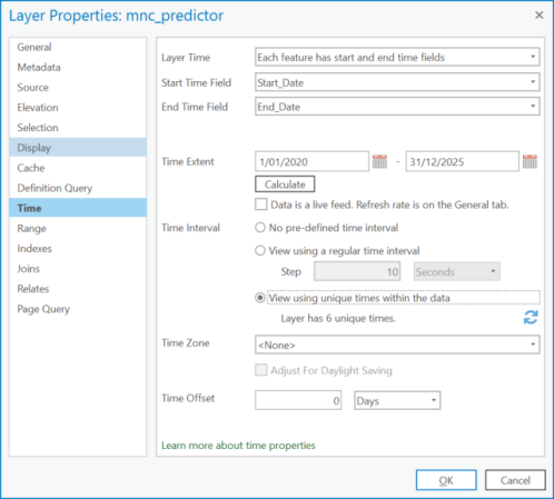
Time Enable the Layer
If Start Date and End Date were added to the data then Time Enable the layer via the layer properties option 'Time'.
The screenshot below shows the selection of the 'Layer Time' option to 'Each feature has start and end time fields". Once selected you will be able to set the 'Start Date' and 'End Date' fields.
For 'Time Interval' choose the option 'View using unique times within the data'
Once set, apply the changes by selecting the 'OK' button.
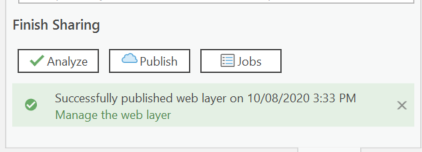
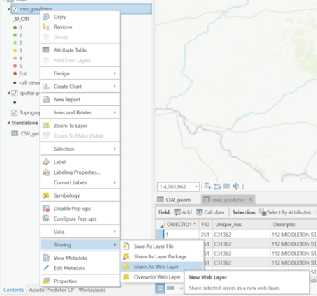
Publish to ArcGIS Enterprise
The layer menu option ‘Sharing’ can be used to ‘Share as Web Layer’.
This uploads the layer as a new feature Service in ArcGIS Enterprise. It requires the user to be signed-in to ArcGIS Enterprise.
On completion of the upload, the new layer can be viewed in ArcGIS Enterprise.